Lab 4A: Cone Follower
Introduction
In Lab 4A, we were tasked with making our robot detect a cone with its onboard cameras and park itself a fixed distance away from the cone. We were able to accomplish this by applying computer vision algorithms and building proportional-derivative and pure pursuit controllers. By processing a stream of images from the camera, the robot can determine the distance and angle to the cone. Our controllers use these as inputs to maintain the required distance from and angle towards the cone. Here is a link to the github repository with the code for this lab. And here is a link to the Google Slides for this lab.
Cone Finder
Accessing Image Data
Our first step in this lab was to access the images taken in by the zed camera. Our zed camera publishes a rosmsg of type image_msg on the /zed/rgb/image_rect_color topic. We wrote a subscriber for the zed camera in order to obtain the contents of this message. We then used cv_bridge to convert the image_msg to a cv2.
Cone Detection
Our goal in this part is to detect the cone, and measure the robot’s distance to and angle from the cone.
Approach
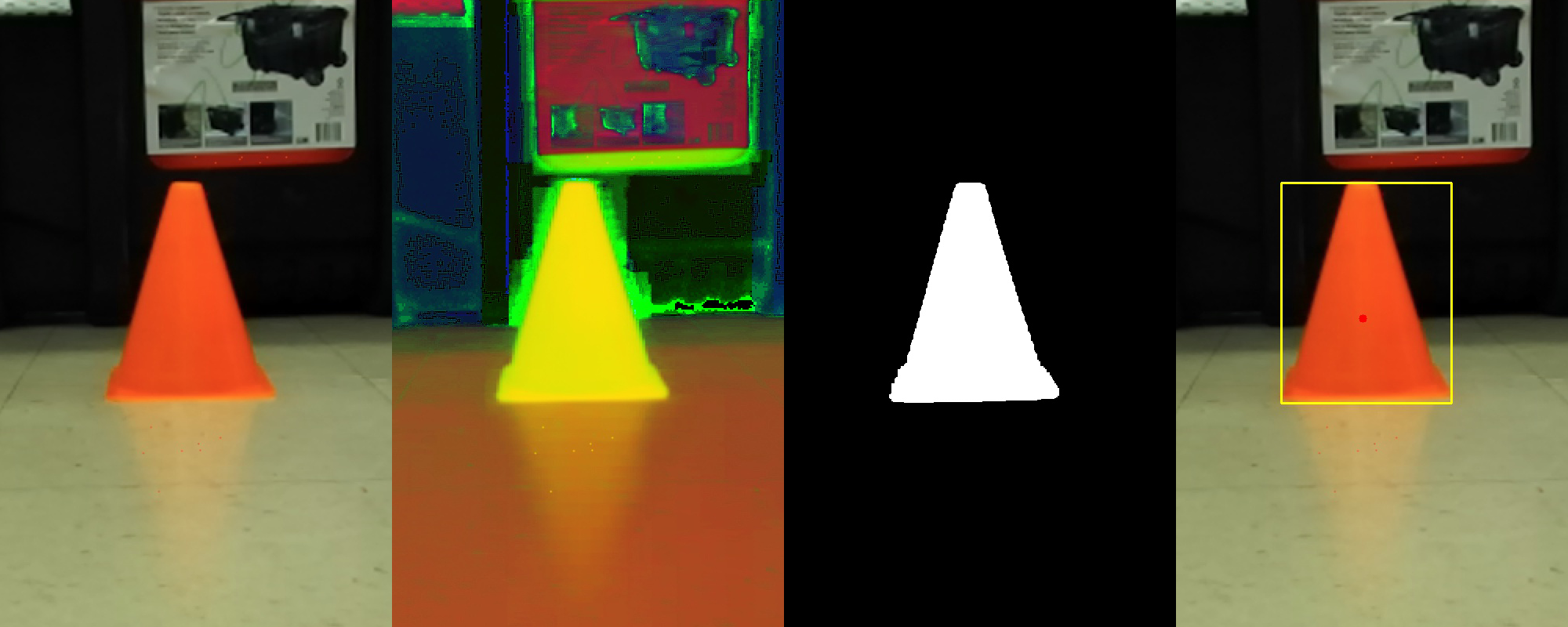
The camera uses RGB images natively, but we chose to map the camera images to HSV space, which uses hue, saturation, and brightness values to display the pixels in an image. In RGB space, the color of the cone is very dependent on ambient lighting conditions, while in HSV space, the cone’s hue value is more consistent across different lighting conditions. We decided that HSV would allow for more robust operation.
We decided to use color matching to detect the cone. Our code scans the image for sets of adjacent pixels within a certain hue interval, corresponding to the cone’s color. It then picks the largest ‘blob’ of such pixels as our cone. Our goal was to command the robot to move towards the blob, until the blob was placed at the center of the camera image and the blob was the correct size, corresponding to a closeby cone.
Implementation
We implemented our approach with the following steps: First, we created a method in the cone_finder.py script to determine where the cone is relative to the car, using the ZED camera images. It first maps the image to HSV space, then looks for each pixel within the HSV range that corresponds to the cone. It filters the image noise with cv2.erode and cv2.dilate methods from cv2, an openCV Python library, to remove random isolated pixels that might fall in the desired range but are not from the cone. It then uses cv2.findContour to generate contours around every collection of pixels that falls within our desired range. This procedure yields a series of contours in our image; we take the largest of these to represent the cone.
Parking our car in front of the cone involves two steps. First, our robot must determine the correct distance from the cone, which involves examining the blob in the vertical dimension. Then, it must center itself front of the cone, which involves examining the blob in the horizontal dimension.
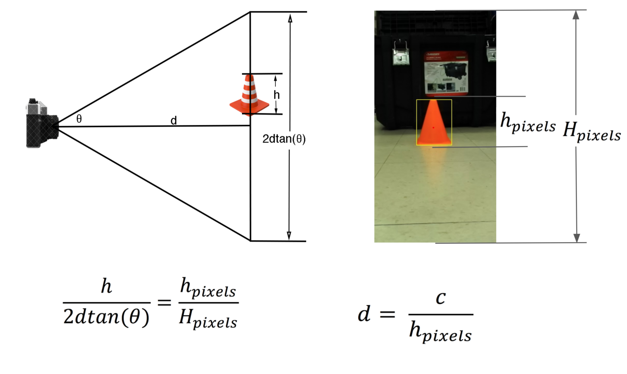
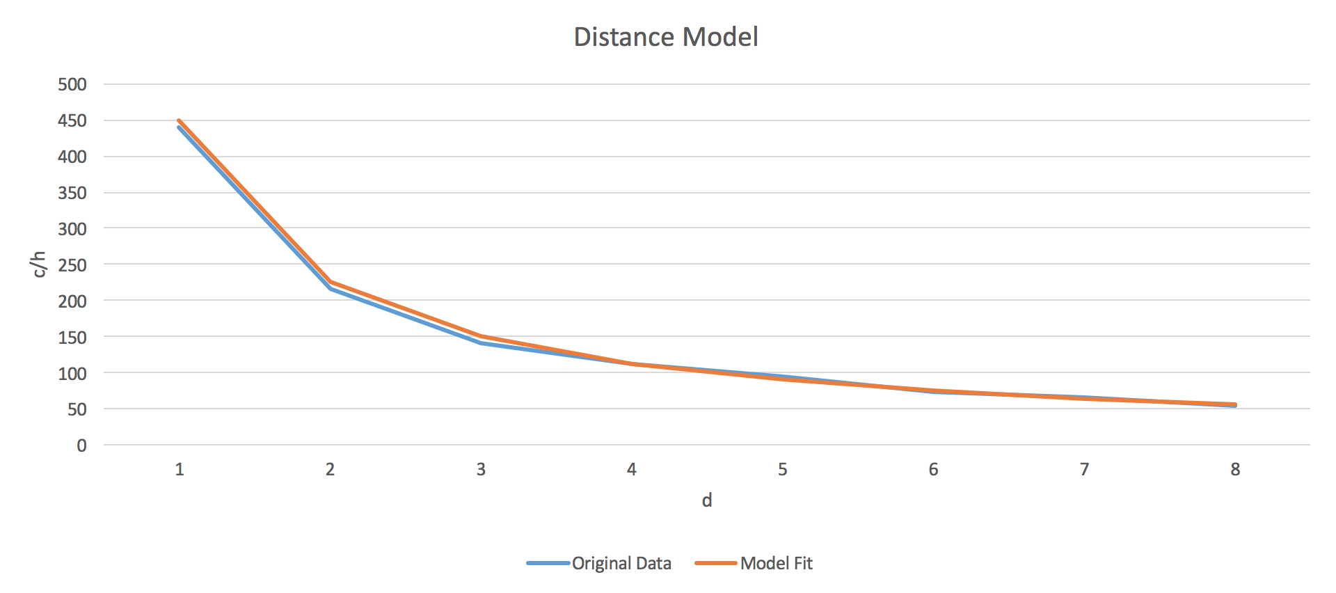
Our robot uses the perceived height of the cone ‘blob’ to estimate the distance from our camera to the cone. To map blob sizes to distances, we took a series of test images of the cone at varying distances, then measured the corresponding sizes of the resulting blobs. From these experiments, we generated a distance coefficient that allowed us to estimate the distance to the cone from a blob height measurement.
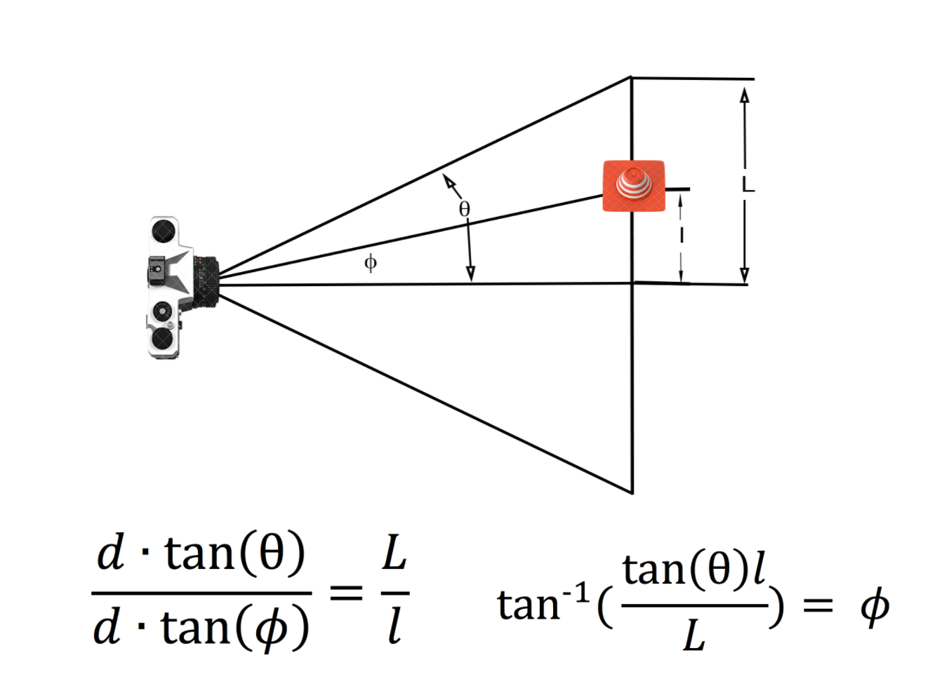
The next step is checking whether the cone is centered. To determine the horizontal position of the blob, we used the cv2.moments to find the center of the mass of the cone blob. By comparing the center of mass of the cone to the horizontal center of the image, and combining this with the distance estimate we just made, we calculated the angle from the robot to the cone.
We then saved the distance and the angle to the cone to a ROS message and published it. The controller is subscribed to the message and processes the distance and angle to the cone in order to move the robot.
Results
Our approach and implementation worked very successfully within the 10m range scale and under proper lighting conditions. However, when the cone was more than 10 meters away, the contour was too small to be detectable by our code, and the cone detection failed. Additionally, when the environment was very dark or there was high sunlight behind the cone, the hue changed beyond the interval we set, and the cone detection failed. We considered removing erosion and dilution to smooth the image, hower that would leave noise in the image that would hamper the contour detection.
Control For Parking
Our goal in this part is to park the car in front of the cone at a half meter distance.
Approach
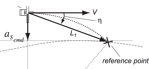
We decided to try out both the geometric Ackermann model with pure pursuit and a proportional derivative controller and test which one performed better. The geometric Ackermann model with pure pursuit, as described in the lecture, detects a velocity and angle towards the reference point through the path of a circle arc. The proportional derivative controller is the same model as we used in the previous lab to detect and follow a wall.
Implementation
Our controller, configured in the cone_follow.py and cone_park.py scripts, is subscribed to the /controller_info topic and receives two feedback values: the distance and the angle to the cone. Cone_follow.py sets the steering angle while cone_park.py sets the forward velocity; they then publish the steering angle and velocity to the high level mux. In conjunction they are able to continuously place the car at the correct desired distance from the cone.
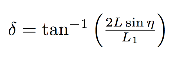
In cone_follow.py, we implemented a geometric Ackermann model with pure pursuit controller that takes in the horizontal error and angle of the cone position and plans the resulting desired trajectory. This uses the horizontal distance to calculate the steering angle with the following formula, where L is the distance between the front and back wheels of the robot, L1 is the distance to the cone, and η is the angle between the vertical line and the line to the cone from the robot.It then publishes the steering angle and the distance to the high level mux.
We also implemented a proportional derivative controller. The PD controller uses the distance and angle error, the angle derivative, and the error gains that we calculated for Lab 3 to dynamically update the steering angle of the robot.
In both cases, the speed parameter is determined by the safety controller to account for the distance to the goal. The steering angle calculation is smoothed by averaging the five most recent steering angles to prevent erratic motion.
Cone_park.py is a proportional controller that subscribes to the distance and angle message, and uses the remaining distance and approach velocity to the cone to determine the speed. Since there is a maximum allowed speed, the robot never goes too fast even if it is far from the cone. The speed parameter is set so that the robot stops when it is half a meter away from the cone.
Results
Both approaches were successful with some differences in the robot motion. With the Ackermann model, the robot followed an arc-shaped path to the cone, and parked at a closer vertical and horizontal distance to it. The arc-shaped path was slightly longer than the PD path. There wasn’t significant overshoot and the robot could stop at an approximately 0.5 meters distance. When the cone was pushed closer to robot, the robot moved backwards facing the cone through an arc-shaped path.
With the proportional derivative controller, the robot followed a straight line towards the cone until it got close enough to adjust its movement more accurately. There wasn’t significant overshoot and the robot could stop at an approximately 0.5 meters distance. When the cone was pushed closer to robot, it first drove backwards facing away the cone, which would become a fail case once the robot changes its direction too much away from the cone. We changed the backward motion steering angle to its negative to adjust for keeping the cone in the camera sight while moving backwards.
There weren’t any failures, as long as the cone remained within sight of the robot and was not too far away. When the robot was placed beyond the ten meter range dictated, it became too small for the camera to successfully detect and resulted in erratic behavior.
Lab 4B: Line Follower
Introduction
In Lab 4B, our goal is to make our robot detect a line with its onboard cameras and drive itself along this line. We used similar computer vision algorithms as used in Lab 4A to detect the line, then tested multiple controllers to get the robot to stay on the line.
Line Finder
Approach
In order to follow the line, we needed information about a point on the line closer to the robot and one farther away.
We needed to determine the distance to the points we found on the image. Due to perspective, points that are farther away are higher up on the image. We used this effect to determine the distance to a point on the ground.
The onboard zed camera has two cameras: a left and a right camera, defaulting to the left camera. Only listening to the left camera caused the robot to center itself on the line relative to the left camera, instead of the middle of the robot. In order to correctly center the robot on the line, we listened to both the left and right cameras and ran line detection on both images, then averaged the results.
Implementation
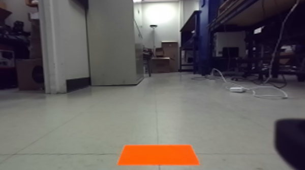
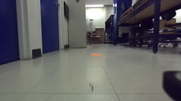
In order to find a point that is on the line near the robot, we used the same object detection algorithm described in cone detection; however, we only look at the bottom quarter of the image. To see a point that is on the line far from the robot we used the same algorithm but we only looked at one eighth of the image, directly above the center.
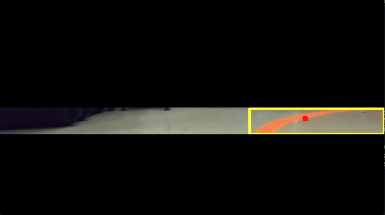
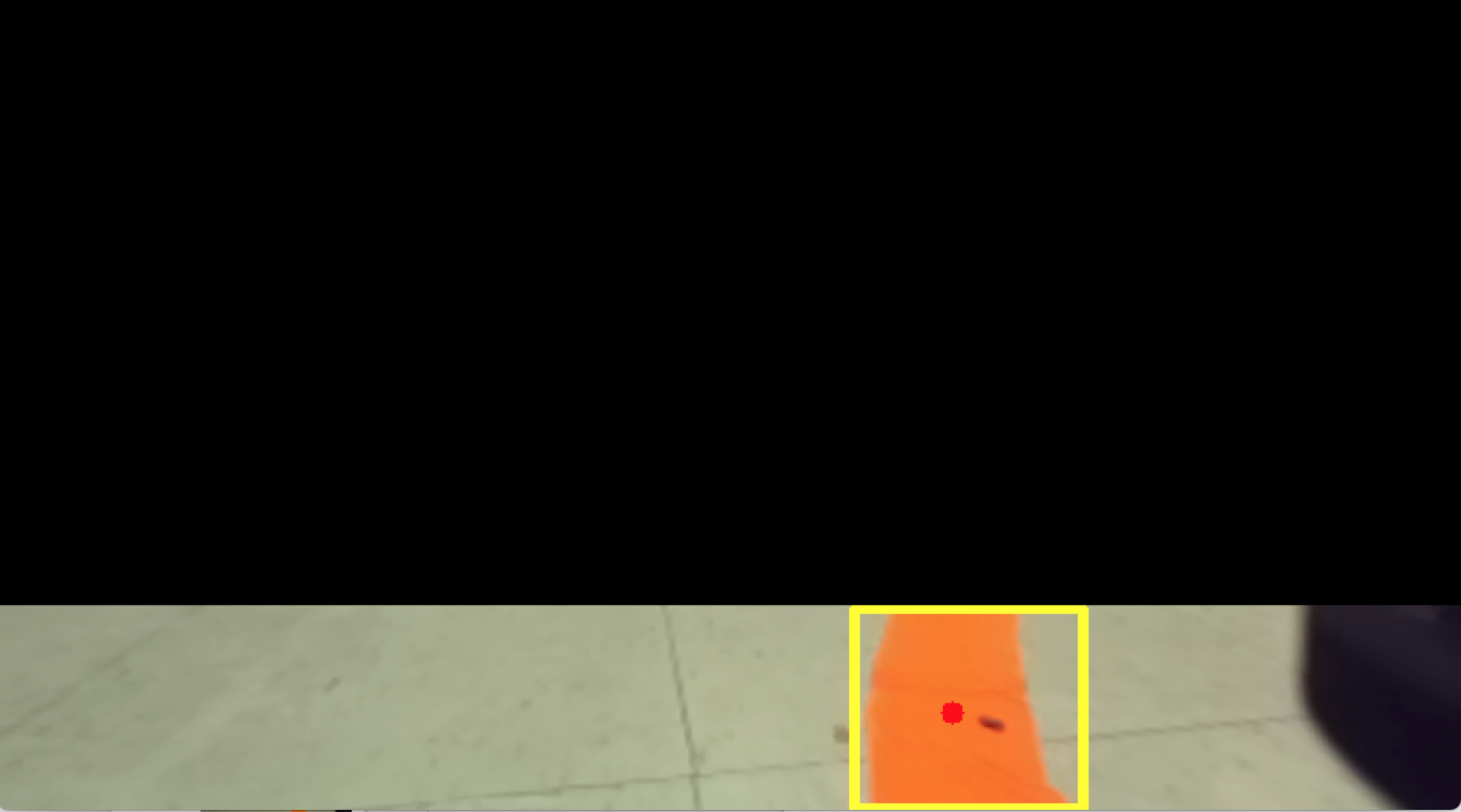
We created a function to calculate the distance to a pixel using the vertical height of that pixel. We accomplished this by taking six samples at various distances, and using the algorithm described in cone detection to find the the center of the orange blob. Then, we created a regression model based on the distances and vertical heights from the images,which resulted in the equation d = .02*e^(.01y)
Line Follower
Open Loop Control
Approach
The goal of open loop control was to create a feedforward controller which instructed the robot to follow the line. Since the line is a circle, we set a constant speed and steering angle.
Implementation
We wrote our open loop controller in the openloop_circle.py script, which continually drives the robot in a circle. The two variables we set were a steering angle of 0.225 radians and a speed of 0.65 m/s, allowing us to complete four revolutions per minute. We arrived at these values through a few trials in Gazebo, then refined them using trials on the real robot. At the time of testing the open loop controller, our robot was a bit damaged and could not reach high speeds, so we settled on a relatively low velocity for the open loop controller.
Results
We were able to drive the robot in a circle five times before it became clear that this was reasonably stable and would not crash into the center obstacle any time soon. Since this is a feedforward controller, we know that we cannot eliminate all error in the real world. That error will accumulate and eventually veer the robot off course.
Setpoint Control
Approach
Setpoint control utilizes a PD controller that focuses exclusively on the bottom of the image and instructs the robot to follow the line, minimizing the angle from the robot to a point on the line ahead.
Implementation
The line finder script returns the angle to a point on the line near the robot, to which we subscribe. We then use proportional-derivative control to minimize that angle and publish a constant speed. We tested the controller on the robot to determine values for the two necessary gains, Ka and Kd, which resulted in smooth line-following. We found that a good Ka for our robot was 0.5 and a good Kd was 2.0.
Results
Our robot was able to drive on the circle indefinitely (or until the battery ran out) even with disturbances. We tested its response to disruptions by nudging it with our feet as it followed the line and observing its reaction.The robot successfully achieved speeds of 1.3 m/s which yielded 8 revolutions per minute.
Trajectory Tracking
Approach
Trajectory tracking (or pure pursuit) uses the geometric Ackermann model to direct the robot towards a point on the line farther away. In order to do this, we used the distance and angle to a point farther away than with previous controllers.
Implementation
TThe line finder script returns the angle and distance to a point on the line farther from the robot as well. We subscribed to that angle and distance and used those parameters, along with the length of our robot, in the geometric Ackermann equation to determine the proper steering angle for the robot.
Results
Our robot was able to drive on the circle indefinitely, responding well to disturbances (as described above). The robot achieved speeds of 1.6 m/s which yielded ten revolutions per minute. However, with pure pursuit alone, the robot focused too far into the future and settled on a path within the boundary of the circle instead of around the perimeter. We decided to implement a fourth controller that combined two approaches to remedy this issue.
Hybrid Controller - Setpoint Control and Pure Pursuit
Approach
Our final controller was designed to fix the issue inherent to pure pursuit, as well as maximize the velocity of the car around the loop. In order to accomplish this, we decided to use both setpoint control and pure pursuit, aggregating the results. Pure pursuit is designed for thinking ahead and our setpoint control is designed for short term results; it seemed logical combining the two would result in the best behavior.
Implementation
Our final controller utilized both the pure pursuit and fixed point calculations already done, running both scripts and then using a weighted average. The higher the velocity commanded, the more heavily it weighted pure pursuit, since fixed point was more reliable at lower speeds.
Results
Our robot was able to drive on the circle, following on the line instead of inside it, indefinitely even with the aforementioned disturbances. The robot was able to reach speeds of 1.9 m/s, which yielded 12 revolutions per minute. We did not want to test the robot at any faster speeds since there were bystanders next to the testing circle and we did not want to put anyone in harm's way.