Introduction
Our goal for this lab was to implement an algorithm to plan trajectories through a map of the Stata basement and then use pure pursuit to follow this trajectory. The first piece was writing a planning algorithm that interprets the map given to it and finds an appropriate path through the environment, cognizant of the walls and careful of sharp corners. The second piece of the lab was trajectory tracking, where we first created a fake path for the robot to follow (for testing purposes). We then implemented pure pursuit to navigate along the path, with a safety controller assuring that the robot does not run into anything. The last piece was to combine the two parts, allowing the robot to find a path through the environment and follow it safely. Here is a link to the github repository with the code for this lab. And here is a link to the Google Slides for this lab.
Path Planning
Planner
Our goal for the path planner is to return a smooth, accurate path in a reasonable time frame such that the robot is able to follow it successfully in the real world.
Approach
The first piece of creating the path planner was to gather information from the map provided and alter its representation into a useful format. The map was reshaped and inverted before being eroded. This erosion process made the halls in the map appear narrower, so that the path determined from the map has a reasonable safety factor, ensuring the robot does not get too close to walls or attempt to cut corners. An additional safety mapping was created, giving the distance to the nearest wall from each point. We implemented three different methods of finding a path from our robot to our goal location: A*, A* with circles, and RRT. Then we checked the performance of each method to compare the results and determine which would work best for us in the tunnels with the actual robot.
Implementation
Our implementation is found in path_planner.py. We first shape the information from the map into a square numpy array, and then invert it. The map was then eroded with a disk shape of radius one third of a meter, roughly the length of the robot, using the skimage_morphology erosion method. We had to use erosion instead of dilation because we had inverted our map to represent traversable areas with 1 and the walls and non-traversable areas as 0. The distance_transform_edt function was used from scipy to give us a mapping of each point to the distance to the nearest wall. We inverted our map in order to be able to use this function.
For A* search, which is found in our Astar() method, we perform A* search on nodes throughout the map, each of which is a discrete piece of the traversable area. We discretize the map into 0.25 meter squares, and each one represents a search node, where each node’s neighboring nodes represent its children. For our heuristic in this implementation of A* search, we simply use the Euclidean distance between the current position and the goal using the numpy linalg.norm method. Once search terminates by finding a path to the goal node, then we are able to return this path. We implement a class called Node within the Astar method, which allows us to trace out a path of nodes by repeatedly calling the Node class’s getChildren() methods.
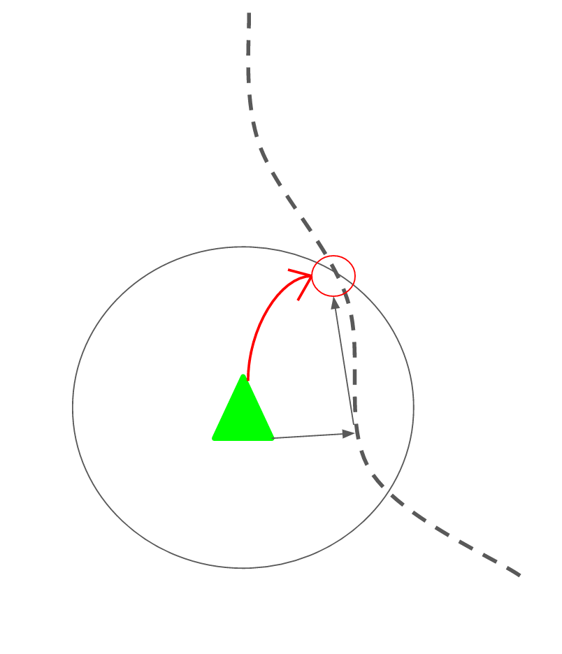
In the Astar_circle method, we implement a method to perform A* search on a collection of circles throughout the map, where each circle represents a search node. Each node that is reachable from another node is listed as one of its children, and the method performs the standard A* search over all the circles in the map to find the goal node specified earlier by self.target_pose. The heuristic used by this method is found in heuristic(), which simply returns the Euclidean distance to the goal node as calculated by the numpy linalg.norm method, same as before with A*. Again, we implement another class called Node within the Astar_circle method, for use in A* search. A path consists of a series of nodes, and once the search terminates we can trace out a path by using each node’s call to getChildren().
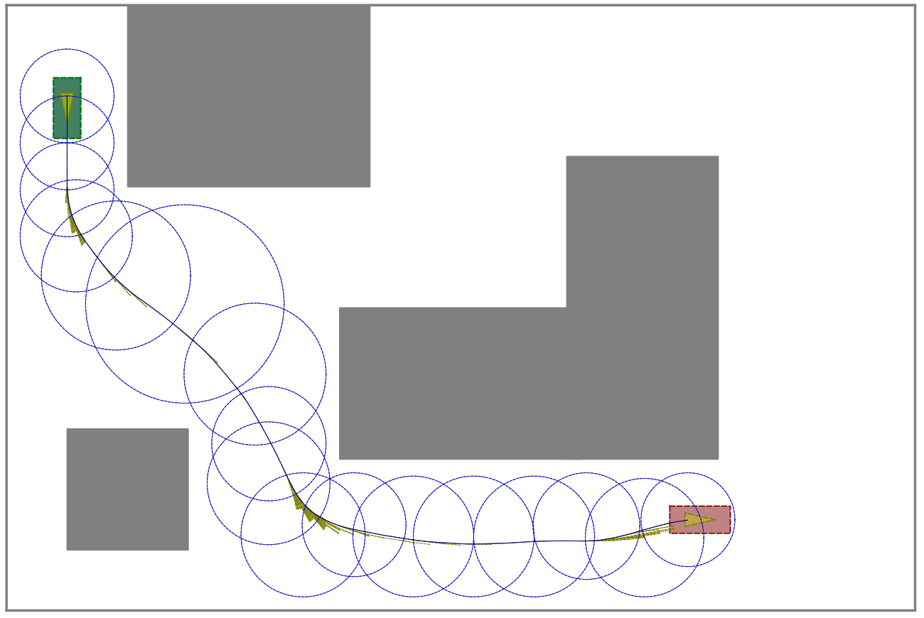
an example of how A* in circular space works from (1)
Finally, in RRT(), we implement the RRT (rapidly-exploring random tree) algorithm to find a path from the current position to the goal position. This algorithm adds nodes to the search tree sequentially as it searches, so it does not start with a goal node already specified. Instead, we have a sort of goal ‘condition,’ where if we add a node that is within half a meter of the goal position, we treat it as a goal node through the goal_reached() method. RRT also gets its own Node class. For RRT, each node is given 10 children, and the getChildren() method branches out 10 equally spaced segments from the node. Each of the 10 endpoints from that node is treated as a children, so it is effectively spreading the tree out from each junction with a branching factor of 10. As it discovers more nodes, it adds them to a heap of nodes, and when it adds a node that satisfies the goal condition from goal_reached(), it returns the path to that node through the current tree’s nodes.
Results
When we tested our three methods to find paths, we found fairly different results for each. It took RRT about 8 seconds to find the path to the goal, but the path that it returned was a jagged and inefficient one. This is a common pitfall of RRT, as it is known to converge to a non-optimal solution. Our path was clearly not one that would have been taken by a human operator. However, the computation time of 8 seconds was very reasonable by our standards.
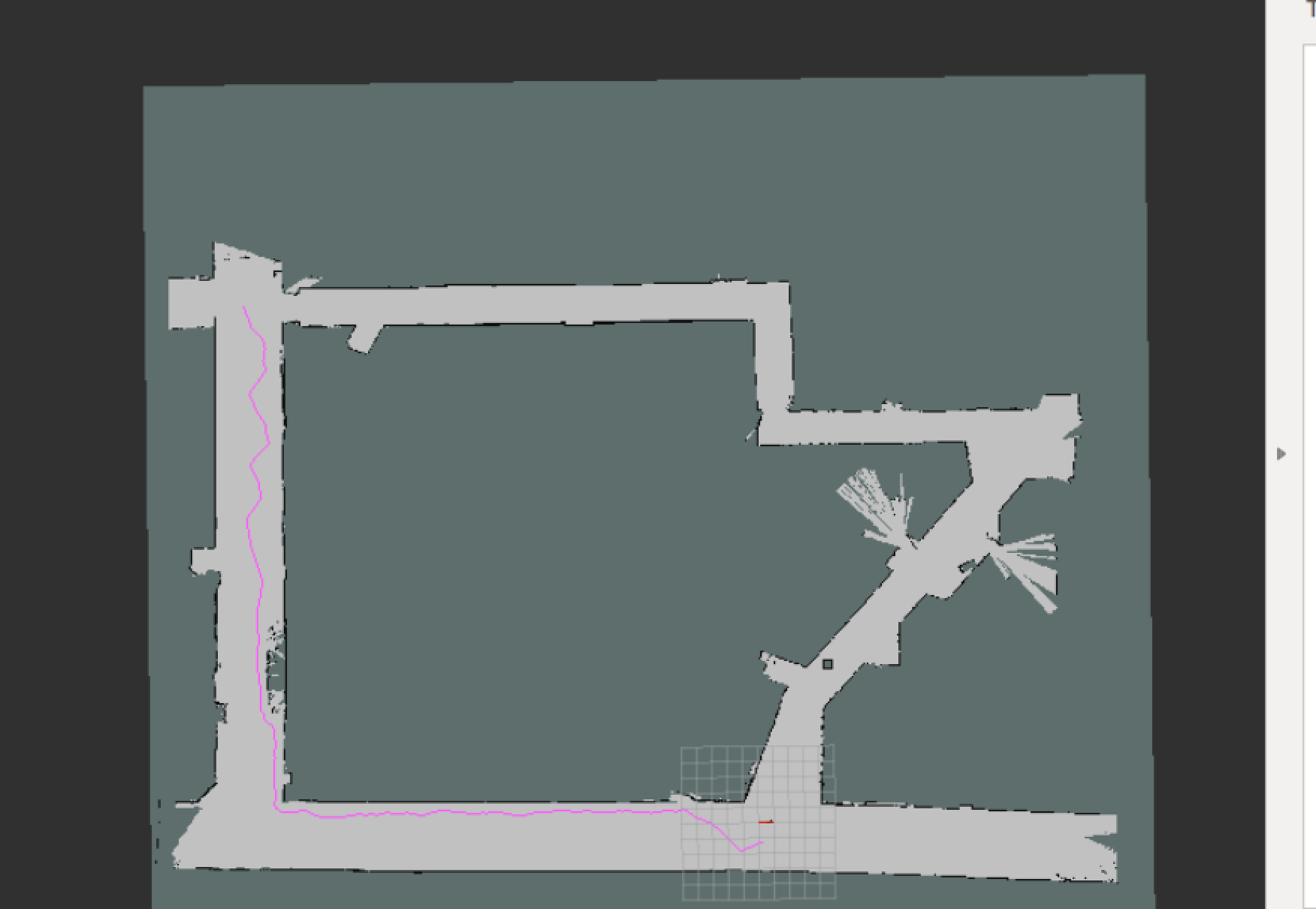
path obtained from RRT
Plain A* on the discretized map ran in slightly less time (about five seconds), but because of the implementation of neighboring nodes and discretization resulted in a path with sharp right angle turns only.
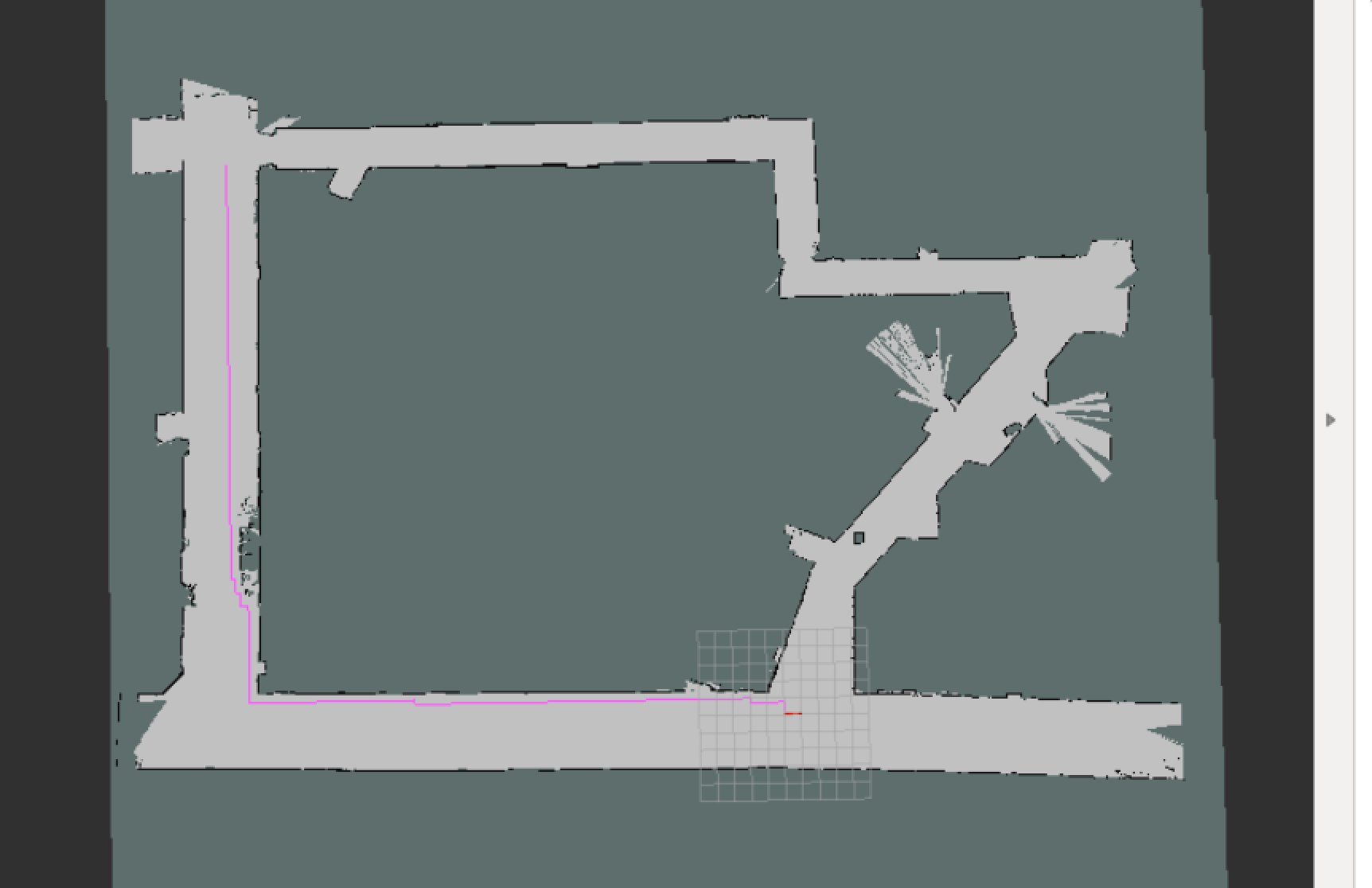
path obtrained from A*
A* with circles gave us a very smooth path that was also efficient, which closely resembled a driving line that would have been taken by a human. The tradeoff, however, is that A* circles took about 80 seconds to complete because of the difficulty of computing its heuristic.
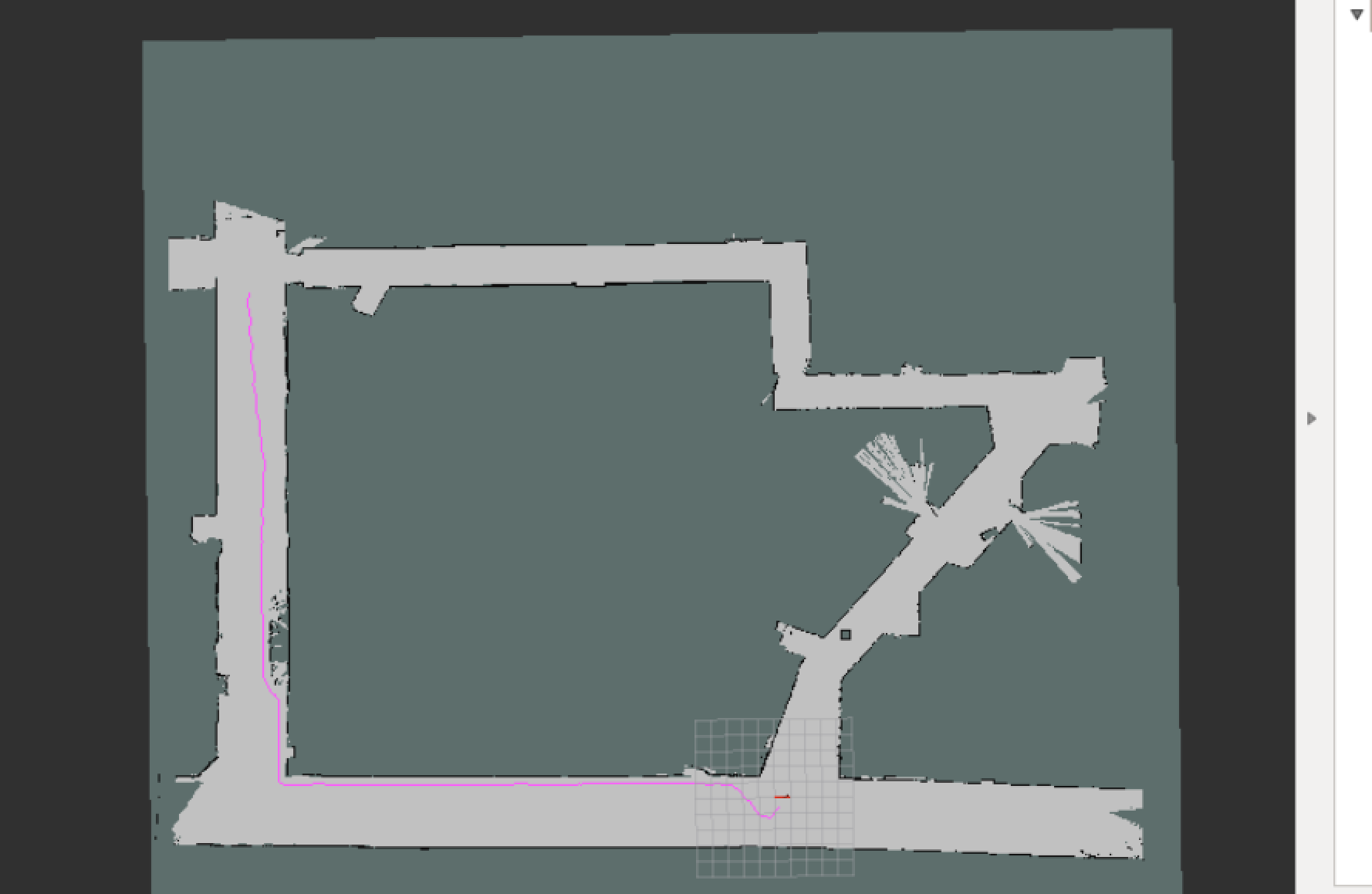
path obtained from A* in circular space
Trajectory Tracking
Our goal for the trajectory tracker is to safely and accurately follow the path given to the function using pure pursuit.
Manual Path
The manual path is a series of line segments the robot can practice following using pure pursuit. This path was created by opening the basement map in Gazebo and placing points around in a rough path; the measurements produced by these points were saved as an array.
Pure Pursuit
Approach
Trajectory tracking was implemented using pure pursuit, which detects a velocity and angle towards the reference point through the path of a circle arc. First, the point on the parth nearest to the robot’s pose is determined. The pursuit target is found by going through the line segments of the path ahead of this point until a segment is found that intersects with a circle of radius determined by the look-ahead distance and centered on the position of the robot. This method was developed with the help of the Pure Pursuit Hints note on Piazza (2). This ensures that the robot will nearly always pure pursuit towards a point forwards on the path.
Implementation
The pure pursuit method is implemented in follow_path() in path_follower.py. The method first determines the robot’s position in terms of x,y, and theta, and then uses the find_nearest_point method to find the nearest point on the path from the robot. The find_nearest_point method iterates through all the points on the path, finding the distance to each one and returning the minimum. The remainder of the path (following this point), as well as the robot’s position and the fixed look-ahead distance of two meters, is then used to find the pursuit target. The find_pursuit_target method iterates through each segment in the path ahead of the nearest point and determines if it intersects the circle of radius look-ahead distance centered on the robot using geometrical calculations in find_intersection. We used an existing implementation from StackOverFlow for finding the intersection points (3). The vector and angle towards the target are calculated, and the pursuit angle is then determined as the difference between the current orientation of the robot and the angle towards the target. The steering angle is calculated using the pure pursuit equation and published to the robot, with a constant velocity of one.
Results
To test our path follower modularly without the path planning system, we created a path on RViz manually. In testing our system, we encountered one issue with the path following algorithm when it was integrated with the path planner due to problems with the trigonometric calculations. Arctangent is used to determine the angle between the robot pose and the target location in the pure pursuit model, but it encountered error because atan() cannot differentiate between angles in the 1st and 3rd or 2nd and 4th quadrants. This was resolved by using atan2() which adds pi to the result of atan() if the cosine of the angle is negative. The pure pursuit method worked smoothly.
Integration
The goal of the integration is to plan a path on the tunnel map and follow the path while avoiding collisions.
Approach
We put our path planner and trajectory tracking pure pursuit algorithm together while integrating the safety controller to prevent the robot from colliding with objects or walls.
Implementation
The path follower subscribes to both the path planner and the localization script to obtain the path and robot pose. Given this information, the find_nearest_point method returns the index of the nearest point in the path to the robot so that the find_pursuit_target method can look ahead of that index for the intersection on the path. After this point is used to determine pure pursuit commands, the speed and steering angle commands are published to the high level mux which then sends the commands to the robot. If the car gets too close to a wall, the safety controller (which subscribes to the high level mux and publishes to the low level mux) overrides and stops the car.
Conclusion
Despite being a difficult lab, the overall process went smoothly, resulting in a functional path planner and trajectory tracker that worked well in the simulation, though it had difficulty working on the robot. To maximize our efficiency, we worked on the path planner and the trajectory tracker simultaneously, dividing into two teams. The trajectory tracking team used the manual path they found in simulation to test their results and the two aspects were later combined for real-world, real-time planning and execution of a path. This lab occurred over a short period of time and was technically challenging, which resulted in a lot of work being done in the last two days. The team pulled together and put in many hours in order to ensure we had a working result.
On the technical side, we learned how to implement the path planner algorithms and integrate with our trajectory planning. Path planning is a prevalent problem with several real life use cases, and we think that we can now better reason about what kind of trade-offs different path planning algorithms have.
References
(1) Chen, Chao, Markus Rickert, and Alois Knoll. "Combining space exploration and heuristic search in online motion planning for nonholonomic vehicles." Intelligent Vehicles Symposium (IV), 2013 IEEE. IEEE, 2013.