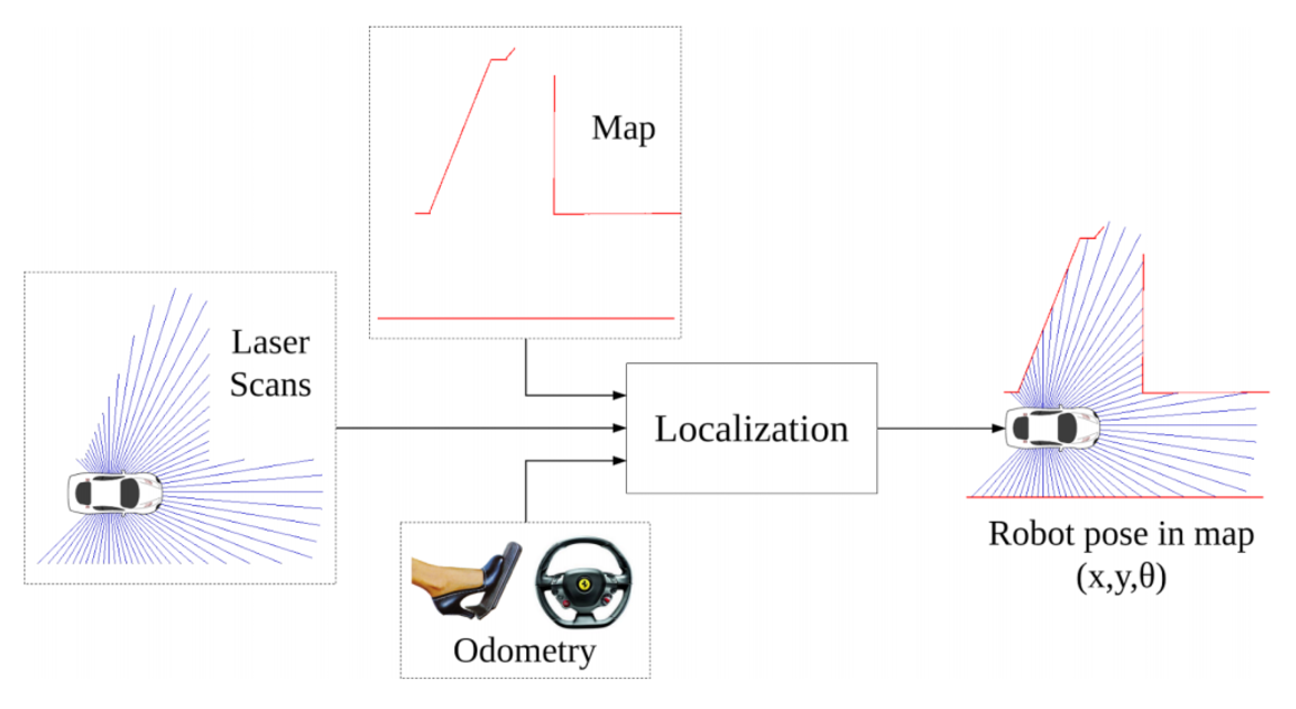
Introduction
Our goal for this lab was to implement Monte Carlo Localization on our robot. To do this, we started by writing the MCL algorithm and testing in simulation, refining using Gazebo and RViz. Next, we demonstrated the functionality of the algorithm in the physical world by uploading it onto the robot and driving it around in the Stata basement. Lastly, we visualized the results of our localization algorithm using tools in ROS in order to improve upon our algorithm.
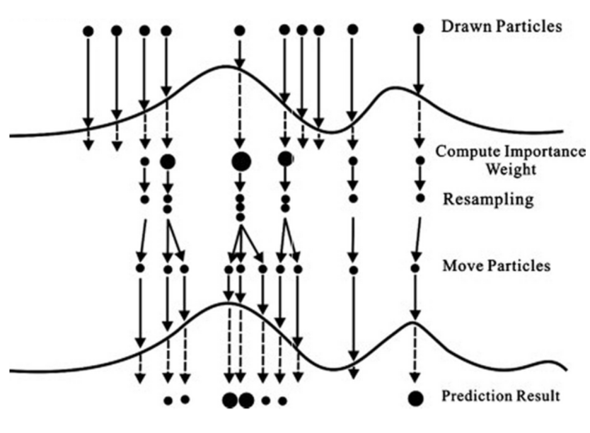
Our MCL makes use of a particle filter, found in particle_filter.py. This particle filter consists of 3 components: a motion model, to track the actions taken using odometry and apply them to the belief state; a sensor model, to refine the belief state based on sensor data; and a particle resampling stage to generate a new proposal distribution using the Monte Carlo sampling method.
Here is a link to the github repository with the code for this lab. And here is a link to the Google Slides for this lab.
Particle Filter
Motion Model
Our goal in this part is to implement a motion model, that would use odometry data with random noise to update our belief state based on our actions.
Approach
Our approach to the motion model is as follows: given our current belief state, we take an action and apply it as a transformation to our belief state. We then add some Gaussian noise to the belief state we get post-transformation, to account for real world imperfections such as noise in our sensor (such as imperfect LIDAR scans) and in our odometry (such as wheel slippage). For our noise, we use a Gaussian distribution with a standard deviation that is proportional to the size of our action, since theoretically a larger action has the potential to introduce a larger amount of noise to our system. We also add a noise from a Gaussian distribution to be applied after the action. We then apply this noise to our belief state to arrive at our new collection of possible locations and orientations.
Implementation
Our implementation of the motion model is found in the motion_model method, which is defined in particle_filter.py. We create a Gaussian distribution centered at 1.0, with a standard deviation of 0.01. When we multiply our actions with this distribution, we get action values with noise added proportional to the size of our action. We then generate the noise to be added after we take our action. We begin by choosing the Gaussian noise; using distributions centered at 0.0, with a standard deviation of 0.05 for the x and y positions and the angle. We chose to use constant standard deviation for this noise because it seemed to work just as well as proportional with experimentation, so we decided to go with the simpler solution. Our belief state is represented as a cloud of three-dimensional points, each of which contains a set of (x, y, theta) coordinates that represents a current possible position and orientation of our robot. The action applied to our position and orientation state is represented in self.action as a numpy vector, so we apply the appropriate trigonometric functions to properly transform each set of x and y coordinates in our belief state. We also apply the angular orientation update. Lastly, we add back the random error that we computed earlier, giving us a new belief state that has had the action applied to it and includes Gaussian noise. This creates a new cloud of particles that is the result of applying our action to the previous particle cloud, along with some added noise. Each of these new clouds is a possible position of our robot, which we will then refine with data from our sensor.
Results
Our motion model based on odometry worked very well. The particle cloud at RViz followed the robot’s actions in Gazebo with high accuracy. The particle cloud did not spread too much, indicating that our model has high precision in its estimations. These observations hold true in all different directions and possible robot angle orientations.
Sensor Model
Our goal of the sensor model is to apply probabilities to each point of the belief state. To accomplish this, we compare actual laser scan data with the ray cast and assign weights to each point in the belief state.
Approach
Our approach was to first take the noisy particle positions found previously as a result of applying our motion model, then refine them by using the data from our laser scanner. From a high level, the approach is to get a raycast from each of the points in our belief cloud, by placing the particle cloud in our map and calculating the distances we should theoretically measure from each angle at each particle. We then take data from our actual laser scanner, which gives us another set of distances at the same corresponding angles. We can then compare the actual scan data to each raycast in our theoretical belief cloud, and obtain an error metric for each point. From this error metric, we can calculate the probability of each location being the actual location of our robot based on the size of the error, thus giving us a probability-weighted cloud of points.
Implementation
To implement the sensor model we created a probability distribution similar to the one described in the lab instructions that gives the probability of getting a certain measured distance, given a certain ground truth distance. The distribution takes the following laser scan measurement cases into account: detecting a known obstacle, detecting an unknown obstacle, missing a measurement, and getting a random measurement. We accomplish this by respectively adding a distribution centered at the measured known obstacle, a slight ramp increasing towards the robot, a high value for the maximum distance, and a uniform distribution with a small value. We then normalize them sum of all these distributions. The distribution we used can be seen in the figure below.
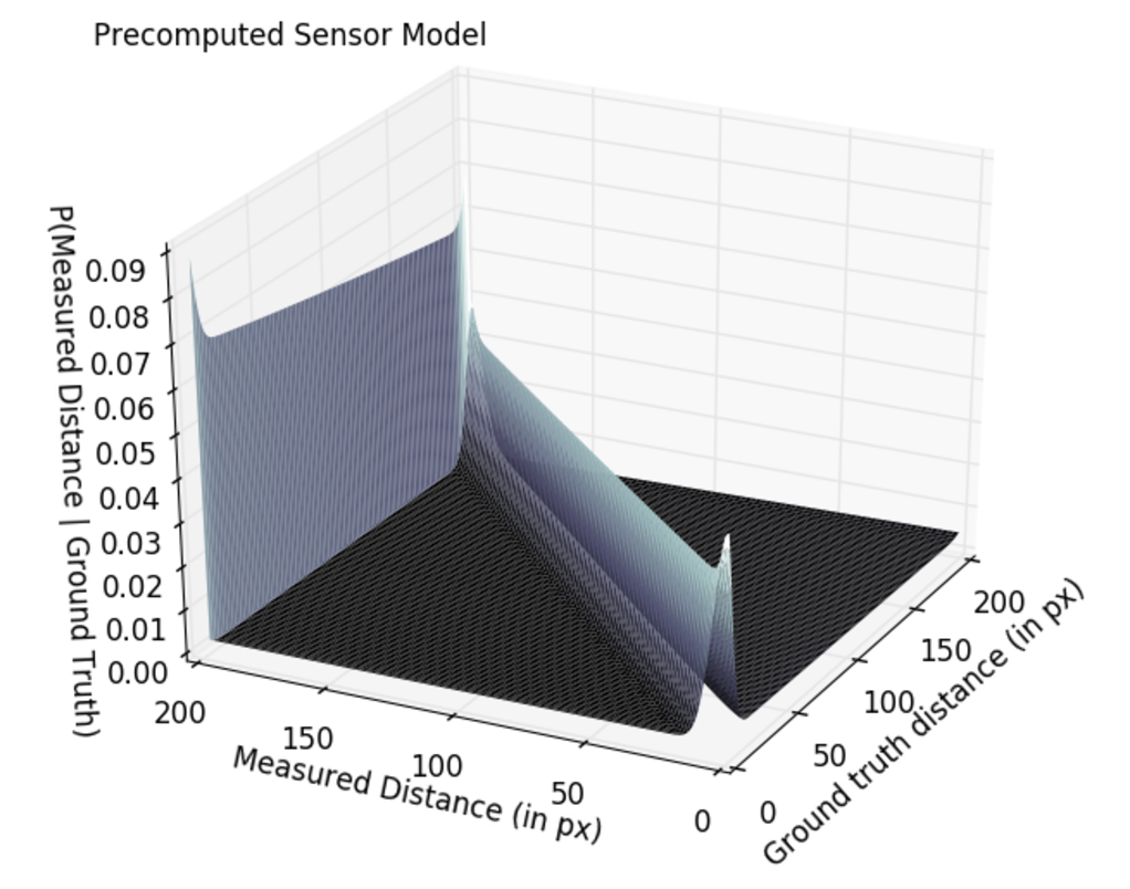
When we were creating the probability distribution, we gathered actual laser scan data from the robot at measured distances that we knew, and calculated the mean and standard deviation of the recorded distances. We found that the standard deviation of the laser scan data was small, and for the most part the data was very accurate, so we incorporated this into our distribution. However, we suspect that the data might be slightly less accurate when the robot is moving, particularly if it is moving at high speed. Unfortunately we couldn’t measure this scenario, because there was no way for us to know the actual distance of the robot to the wall if the robot was in motion.
We also tested the variance of the laser scan measurements for all possible angles to account for measurement faults of the physical system. While the robot is standing, there was zero variance in the measurement values, showing that the laser scan measurements are very robust. However, it was almost impossible to measure the variance in the measurements for a specific laser scan angle, while the robot is moving. Even if there would be some measurement error, we did not take that into account.
Once we had the distribution we created a discretized table, so that we could quickly refer to it in order to find the probability of getting each particle’s raycast, given the raycast data we had from the laser scanner. We used calc_range_repeat_angles given to us in range_libc, to create an expanded list of the raycast for each particle. And then we used eval_sensor_model to calculate the probability of each particle using our discretized probability table, and assign weights based on that probability.
Results
The sensor model worked very well. Based on the ground truth, we get a cloud distribution around the location of the robot with an increasing concentration of particles closer to the robot. The angle points to the right direction. When we use point click in RViz to drag the robot to a different random point, the sensor model locates the robot based on the ground truth in a few seconds. You can see this in the video below.
MCL Algorithm
Monte Carlo Localization (MCL) uses particles to represent its belief state and estimate its position and orientation on a given internal map. Our goal in this part is to implement the Monte Carlo Localization (MCL) algorithm with our robot and test it in simulation and the MIT Tunnels.
Approach and Implementation
Our approach was to use our sensor and motion models with Monte Carlo sampling to implement the MCL Algorithm. In the MCL algorithm, the motion model is run to generate the initial pose, the sensor model is then called to assign weights to each of the points, and then the particles are resampled based on the assigned weights. The particle resampling stage utilizes Monte Carlo sampling to generate the new proposal distribution by “randomly” sampling MAX_PARTICLES number of particles from the list where the normalized weight of each particle is used as the probability of being selected. We are then left with the same number of points, but each was resampled based on weights determined in the sensor model.
Optimization
We took the approach of optimizing as the code was written instead of waiting until the very end to improve performance. One of the first and simplest things done was using numpy arrays and functions instead of slower python lists and loops, as per the suggestion in the lab instructions. We also identified the critical paths through the code, most specifically the ray casting methods which are very expensive. We played with different ray casting (range) methods; however, we found that CDDT had the fastest initialization time and worked quite well on the simulation. For the robot we use RMGPU since this was by the best, when using the Nvidia Jetson-TX1 board (GPU). These optimizations allowed for a more efficient (and thus more successful) particle filter, running quickly enough to keep pace with the sensor data being received.
Results
We tested MCL algorithm by running it in RViz and observing the behavior of the robot. The robot worked better in the tunnel system then it did in the simulation. This is probably because the map was made from the tunnel system rather than from the Gazebo Tunnel which is slightly different and probably threw off the sensor model. Robot seemed to be very resistant to noise in the tunnel system and detected the people walking in front of it as well as unknown obstacles such as the robot box on its way.
Simulation
MIT Tunnel
Visualization
As mentioned earlier, we used RViz throughout the lab to help us visualize the particle filter, and nail down any issues in our code. First, we added the Map topic and saved it onto our racecar. We then created the functions visualize, publish_particles, and publish_scan to achieve our visualization. Visualize samples one hundred particles from our particle filter, which is a reasonable number of particles to manage. Publish_particles then publishes those particles to RViz in a PoseArray message. The messages are continuously sent as the robot moves, so that the particles visible in RViz reflect what is happening in real time. Additionally, publish_scan publishes the laser scan data that is received from the robot to RViz.
Conclusion
This lab was an overall success, resulting in a functional Monte Carlo localization algorithm that worked well in the simulation and the MIT tunnels. We learned a lot about using probabilistic methods for robot localization and using maps and visualization methods for robotics with ROS and we learned to work better as a team.
This lab was difficult to coordinate due to the timing of spring break, and the variety of plans made by members of our team. However, we managed to keep each other updated and coordinated well remotely on our progress. Proper communication was one of our goals for this lab to improve on, and we got significantly better at it.
Improving on the last lab, we better communicated our expectations to each other. We accomplished this by talking through different components of the lab. We followed a common media standard for our images and videos, which was an issue during the previous lab.
On the technical side, we learned that we should be aware of package and library update compatibility. The zed_wrapper update by ROS in the middle of the lab. This required heavy debugging since the zed_wrapper update deprecated our code and made it difficult to catkin_make. In order to get around this bug the team had to completely remove zed from src, which was not a problem since this lab does not use the zed camera.